Rose Zhang graduated from the Department of Economics, University of Toronto in June 2023. She is now an MSc student at the London School of Economics.ECO499, Honours Essay in Applied Microeconomics, is a course that enables students to complete an original research paper on a topic of their choosing. The topic must be microeconomic and applied, meaning all papers will involve data and quantitative (regression) analysis. Rose’s paper was awarded the Arthur Hosios Scholarship in Economics for best paper submitted during the 2023-2023 academic year on 6 March, 2024.

Established by the family and friends of the late Professor Arthur Hosios, the scholarship is held by one or more students on the basis of an original research paper that the applicant submitted as part of the requirements of a 300 or 400 level Economics course taken at the University of Toronto (St. George campus), for which the applicant received a credit. The applicants’ work is evaluated based on originality and presentation. There are two awards – one each for the winning and second best paper.

The Impact of Short-Term Rentals on Housing Prices & Rents

 

Abstract

I study the impact of short-term rentals (STRs) on housing and rental prices in the United States, leveraging the fact that many cities in the U.S. have implemented regulations restricting STRs over the past decade. I estimate the effects of these regulations using a state-of-the-art staggered difference-in-differences methodology, and find drastically different effects on home values depending on neighborhood and home characteristics, and insignificant effects on rents. Homes in locations that are more attractive to tourists experienced a 3.26% decrease in value as a result of the regulations, while homes in other areas saw their values increase by 2.82%. Both these estimates become greater in magnitude when only considering effects on smaller homes (1-2 bedrooms) and larger homes (3+ bedrooms) respectively.

1           Introduction

The concept of home sharing or short-term rentals (STRs) has grown increasingly popular over the past decade, particularly with the introduction of online platform Airbnb to the market in 2008. There are currently 6.6 million active listings on the platform worldwide, with over 4 million hosts. (Airbnb Newsroom, n.d.) In theory, peer-to-peer markets like Airbnb should increase economic efficiency – they allow for the allocation of otherwise unused resources, and facilitate matching between buyers and sellers. However, there has been more and more criticism about the negative impacts of STRs that have caused cities around the world to begin introducing STR regulations. The term ‘Airbnb Effect’ has been adopted to describe the increasing home prices and rents in neighborhoods as a result of the success of the platform. Due to this and complaints from local residents, many policymakers are implementing laws to restrict STRs in hopes to increase housing affordability. (Baker, 2020)

In light of all these concerns, in this paper I investigate whether STRs have had a causal effect on residential house prices and rents in the United States. I obtain a comprehensive panel dataset on home value and rental rate indices from Zillow, with each observation at the zipcode-month level. To test for the causal effect, I leverage the fact that many cities in the U.S. have adopted STR regulations at varying times over the last decade. There is evidence that these regulations have proven effective in reducing the number of STRs in affected cities, as I will discuss later in the paper, so these regulations can be used as exogenous variations in STR supply to test for the effects of STR supply on the housing market. I collected regulation data on 110 cities in the U.S., finding their regulation status and effective dates of the regulations if applicable, as well as information on the specific types of regulation. For my analysis, I use the staggered difference-in-differences framework developed by Callaway and Sant’Anna (2021) in order to account for the varying treatment times and heterogeneous group treatment effects.

I first find that these regulations caused a 1.98% increase in overall home values in treated zipcodes in my sample, which is a $5911 increase in the mean value, statistically significant at the 1% level. My estimate on the treatment effect on rental prices was not statistically significant from zero. Both these results differ from those found in the existing literature, but additional analysis shows that the effect on home values can be separated into two different effects based on zipcode characteristics and home types. I find that among zipcodes with high tourism levels, STR regulations in fact caused a 3.26% ($13,766 on average) decrease in home values in treated zipcodes. In contrast, all other treated zipcodes (in zipcodes with low tourism levels) saw a 2.82% ($7824 on average) increase in their average home values as a result of the regulations. These effects are even higher in magnitude when only considering smaller homes in high tourism areas, and larger homes in low tourism areas respectively.

Overall, these results present evidence of both the positive and negative impacts STRs have on home values in a neighborhood. Importantly, I find that the lesser explored negative externalities of STRs can actually decrease home values in zipcodes not catered towards tourists. These findings provide useful insights for policymakers when considering the implementation or amendment of STR regulations, and whether or not the regulations will actually address their concerns. This is especially important for those considering regulations to improve local affordability of housing, as my results suggest that regulations may do the opposite of what is intended in neighborhoods where locals are more likely to live.

2         Literature Review

There is a lot of existing literature focused on the impacts of short-term rentals and home sharing. Those that are most closely related to this paper investigate the effects of STRs, particularly Airbnb, on the housing market. Using different methods for data on different cities, Horn and Merante (2017), Garcia-Lopez et al. (2020), Barron et al. (2021), and Farhoodi et al. (2021) all investigate the effect that Airbnb listings in a neighborhood have on the housing and rental prices in that neighbourhood, and find positive relationships for both. Valentin (2020), Duso et al. (2020), Koster et al. (2021), and Chen et al. (2022) also investigate this relationship, but instead leverage the growing number of short-term rental policies affecting Airbnb and use event study designs to estimate the effect of the policies on the housing market. They all find a negative treatment effect of the Airbnb-restricting policies on home prices and rents, and also that the policies did in fact decrease Airbnb supply. Overall, we can see that the literature on this topic has been consistent in finding results that support the positive relationship between STRs, and home and rental prices.

Other literature on STRs investigate their impacts on other socioeconomic variables. For example, Bekkerman et al. (2022) find that STRs incentivize residential investment. Zervas et al. (2017) and Farronato and Fradkin (2022) investigate the welfare impacts of Airbnb entry in the accommodation market, finding that it has generated millions in consumer and peer-host surplus, while reducing the revenues of incumbent firms (hotels).

This paper adds to the literature by investigating the impacts of STR regulations on the U.S. housing market at a larger scale. Previous research that has used STR regulations for event study designs has been focused on effects in a single city or several cities (and typically very large cities such as New York City, Los Angeles, Barcelona, etc.). However, I have collected regulation data on 110 cities in the U.S. and am thus able to conduct a more comprehensive analysis of these effects across the U.S. In fact, because of the scale of this analysis, I was able to find evidence of heterogeneous effects of STRs on the housing market based on zipcode and home characteristics, which has not yet been explored by the literature. Moreover, I estimate treatment effects using the state-of-the-art staggered difference-in-differences method developed by Callaway and Sant’Anna (2021), which allows for the causal interpretation of my results.

3          Theoretical Framework

3.1         A Simple Search and Matching Model of the Housing Market

In order to understand the potential effects of STRs on the housing market, I considered a simple search and matching model of the housing market. This model was developed by Farhoodi et al. (2021), and is largely based off of models developed by Mortensen et al. (1986), Genesove and Han (2012), and Han and Strange (2015).

Consider a one period model of the housing market where there are B buyers and S sellers. Let m(B,S) be a matching function that outputs the total number of matches in the market. I assume that this function has constant returns to scale, so m(aB,aS) = am(B,S) for any constant a. Then, define the probability that a seller contacts a buyer to be:

where is defined to be a measure of housing market ‘tightness’. Similarly, define the probability that a buyer meets a seller to be:

Call X the value of owning a home, and draw this from distribution F(X − v) where v is a demand shifter for homes. Thus, a higher v would lead to a higher expected value of the property. Call the values of searching for a match for buyers and sellers V ^B and V ^S respectively. Here, V ^S can be interpreted as a seller’s reservation price for selling their home. Finally, define c^B and c^S to be the buyers’ and sellers’ costs of search for a match in this market. Search costs could include the time and energy it takes to find a match, for example. In the seller’s case, it could also include the opportunity cost of not renting the property out while it is up for sale. For a transaction in the market to occur, it must be that X ≥ V ^B + V ^S ≡ y. In other words, the value of owning a home must be greater than or equal to the combined search values of the buyer and seller.

A home price P is determined through Nash bargaining. Define β ∈ [0,1] to be the bargaining power of the seller. Seller surplus is P − V ^S, buyer surplus is X − P − V ^B, and therefore total surplus is equal to X − (V ^B + V ^S) = X − y. Nash bargaining for this total surplus gives equations:

P − V ^S = β(X − y)

X − P − V ^B = (1 − β)(X − y)

=⇒ E[P] = V ^S + βE[X − y | X ≥ y]

For a given interest rate r, we also have the following asset equations on the supply (seller) and demand (buyer) sides respectively. The opportunity cost of the transaction rV ^S or rV ^B can be expressed as a function of the market tightness θ:

rV S = qS(θ)[1 − F(y − v)] · βE[X − y|X ≥ y] − cS	(2)
rV B = qB(θ)[1 − F(y − v)] · (1 − β)E[X − y|X ≥ y] − cB	(3)

The right side of equations (2) and (3) are equal to the expected net surplus from a successful transaction.

3.2         The Effects of Short-Term Rentals

With the simplifying assumptions that supply is fixed and V ^B = 0, Farhoodi et al. (2021) prove that an increase in demand for homes v leads to increased market tightness θ and value of being a seller V ^S, leading to an increase in expected prices. The opposite is also true – a decrease is demand for homes leads to a decrease in expected home prices.

There are two counteracting effects STRs have on the demand for homes that have been considered by existing literature:

1. STRs can increase the demand for homes v in a neighborhood through:
   • Introducing a new potential revenue stream for homeowners
   • Positive externalities of drawing tourists to the neighborhood, increasing revenue for local businesses, and increasing the value of the space
2. STRs can decrease the demand for homes v in a neighborhood through:
   • Negative externalities such as causing noise pollution, a lowered sense of community, and concern for safety

Existing literature has largely found that the first effect dominates the second, resulting in STRs causing rising home prices as well as rents. However, the magnitude of such effects can depend on a variety of factors. For example, the revenue potential of a STR is highly dependent on how attractive the unit is to tourists, as they make up most of the demand for STRs. If a STR is in a location that is closer to tourist attractions and/or the city center, it has more revenue potential and this will likely dominate the effect that negative externalities have on housing demand. Furthermore, since these areas are already dominated by tourists, the negative externalities from additional STRs are likely to be very small considering that aspects like noise and a high volume of tourists (no sense of community) are already expected. On the other hand, those living in quieter, more suburban neighborhoods are likely to have more concerns over the noise and unfamiliar faces STRs bring. Coupled with the low revenue potential of STRs in these more ‘local’ neighborhoods, it is expected that STRs will cause demand for homes to decrease in those neighborhoods.

4           Data

4.1         Short-Term Rental Regulations

STR regulation varies across cities in the U.S. in terms of their implementation date and also the actual form of regulation. Common approaches include requiring the application for a STR specific license, restricting the number of days in a year a home can be rented out in the short term, and restricting the number of STRs a single host can operate. I manually collected information on these regulations through city websites, city-specific STR ordinances, and news articles. I focus on cities in the U.S. with population over 200,000 (medium sized urban cities or larger) to ensure that treatment and control groups in my analysis would be comparable. Additionally, my analysis is limited from January 2000 to December 2019 to avoid any effects from the COVID-19 pandemic that could skew my results.

I report descriptive statistics of these regulations in Table 1. There are a total of 127 of cities in the U.S. with population over 200,000, but 17 cities were removed from the sample as I was unable to confirm the implementation dates of their STR policies, leaving 110 cities for analysis. ‘Regulated’ is a binary variable indicating if there was any type of regulation in that city, and ‘Effective Date’ is the effective date of the STR regulation in months since 2000. We can see that 43% of cities in the sample were regulated between January 2000 and December 2019, and the median effective regulation date is April 2018 (220 months after January 2000). Figure 1 shows the distribution of regulation dates in the sample, and we can see that the earliest regulation was implemented in the first quarter of 2012 and an increasing number of cities have adopted regulations in recent years.

4.2         Zillow Housing Data

I have collected zipcode-month level data on house prices and rents from the real estate information company Zillow. Zillow publishes the Zillow Home Value Index (ZHVI) and Zillow Observed Rent Index (ZORI), both of which are smoothed and seasonally adjusted measures of the typical home value and market rent in a given region. Their website also publishes ZHVI for different home types and sizes: single-family residences, condos/co-ops, and all homes with 1, 2, 3, 4, and 5+ bedrooms. I report summary statistics for this data in terms of zipcodes in the control group and those in the treatment group in Table 2 and Table 3 respectively. Overall, we can see the means and medians in the treatment group are higher than those of the control group across all measures of home value (ZHVI) and rent (ZORI). As this is averaged across the entire sample period, this could be an indication that STR regulation had a positive treatment effect on all these measures, but also brings attention to possible pretrends of whether or not zipcodes in the treatment group already had increasing home and rental prices. I will confirm that this is not the case in the Results section.

Also, it should be noted that the lack of observations for ZORI is due to the smaller time frame of available data (May 2015 – December 2019) compared to that of ZHVI (January 2000 – December 2019).

4.3         Tourism Levels

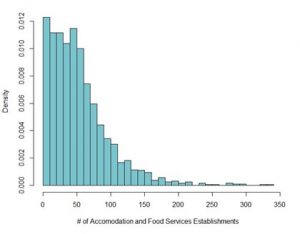
To measure tourism level in a given zipcode, I use Zipcode Business Patterns data from the United States Census Bureau. Using the same method as Barron et al. (2021), I collect data on the number of establishments in the Accomodation and Food Services industry (NAICS Code 72) to proxy for tourism level. I use data from 2000, the earliest year in my sample, to ensure that this measure would not be affected by the treatment in any way. I present summary statistics for this data in Table 4 and plot the distribution of zipcode tourism levels in Figure 2. We can note the high variance of these values across all zipcodes, and that most zipcodes, as expected, have a number of such establishments on the lower end of the distribution.

5           Methodology

5.1         Empirical Model

To estimate the causal effect of STRs on the housing market, I leverage the fact that STR regulations have been adopted in many U.S cities over the past decade. I consider cities that have implemented some form of STR regulation to be treated, and those with no regulations as part of the control group. Then, I can use a difference-in-differences methodology to identify the average treatment effect of STR regulation on the treated zipcodes (ATT) in my sample.

Since STR regulations are determined at the city level and I am using zipcode-month level data, this natural experiment has a lot of variation in treatment timing. This differs from the canonical difference-in-differences setup with only one treatment time, and offers the advantage that the ATT identified will not be biased by any national or global events affecting the housing market. However, there is the added complexity of treatment effect heterogeneity based on the timing of the treatment in a city. Considering this, I use the staggered differencein-differences framework proposed by Callaway and Sant’Anna (2021), which specifically addresses the above mentioned factors of staggered treatment and heterogeneous treatment effects. It also allows for causal interpretation of its results, contrary to the flaws in the twoway fixed effects (TWFE) method recently pointed out by by Borusyak and Jaravel (2017), de Chaisemartin and D’Haultfœuille (2020), Goodman-Bacon (2019), Sun and Abraham (2020), and Athey and Imbens (2018).

The framework is structured as follows: let i denote a zipcode, t the month-year, and T the total number of months in the sample. Define Y_it to be the observed outcome of interest, which is either a measure of home values or rental prices. Define G_ig to be a binary variable equal to 1 if zipcode i was first treated at time g, and 0 otherwise. Denote Y_it(g) to be the potential outcome of zipcode i at time t if it was first treated at time g, and let Y_it(0) be the potential outcome of zipcode i if it was never treated at any time within the sample period.

The relationship between the observed and potential outcomes for each zipcode i at time t is then:

We can see that the above equation incorporates variation in treatment time by defining different treatment groups g, and since potential outcomes are a function of the treatment group, heterogeneous group treatment effects are accounted for. The ATTs, dependent on treatment group g and time t, can be defined as: ATT(g,t) = E[Y_it(g) − Y_it(0) | G_ig = 1]

I report my estimates by aggregating the ATTs into an overall treatment effect θ according to the below scheme, which is effectively a weighted sum. ω_g represents weights proportional to the number of zipcodes treated at time g, and κ₀ normalizes the weights so they sum to one.

5.2         Key Assumptions

The identification of each ATT(g,t) is dependent on several assumptions about the data. First, I assume random sampling of my observations, where the observed outcomes and treatment decisions for all zipcodes i and times t are independent and identically distributed (iid). This is achieved through the use of panel data, which I use in my analysis. I also assume no anticipation of treatment and irreversibility of treatment – once a unit is treated, it remains treated throughout the sample period at the same intensity.

Finally, there is a key parallel trends assumption where, for all i, each g, and all t ≥ g:

E[Yi,t(0) − Yi,t−1(0) | Gi,g = 1] = E[Yi,t(0) − Yi,t−1(0) | Gi,g = 0 ∀g]

In other words, if treated zipcodes were instead untreated, then the change in their outcomes should be the same as the change in outcomes of zipcodes in the control group. This ensures that the estimated treatment effect can be interpreted to be solely caused by the STR regulation and not any other underlying mechanism. Although this assumption cannot be tested, as we do not observe the counterfactuals Y_it(0) in the treatment group, I test for the existence of differential trends prior to treatment which is a good indication of whether or not this assumption holds.

6        Results

6.1         The Effect of STRs on Home Prices and Rents

I first report results on the overall effect of STR regulations on home prices and rents in the U.S in Table 5. The first column shows estimated ATTs with ln ZHVI as the dependent variable, and second column with ln ZORI as the dependent variable. We can see that homes in treated zipcodes experienced a 1.98% increase in value on average as a result of STR regulations, statistically significant at the 1% level. In terms of the mean ZHVI in treated zipcodes, this is approximately a $5911 increase in home value, which is quite economically significant. On the other hand, the estimated treatment effect on the rental index in treated zipcodes is negative at -2.44%, although statistically insignificant. These results contrast with existing research on this topic, which have largely found statistically significant effects of either STR presence increasing home values and rents, or that STR regulations cause decreases in those same measures.

I also examine how this treatment effect evolves over time in Figure 3. Although there exist some minor pretrends in the plot on the left (for ln ZHVI), we can see that the positive treatment effect is clearly not driven by such pretrends and is increasing in magnitude over time. For the plot on the right, treatment effects on ln ZORI, we see no differential pretrends.

Additionally, the point estimates are negative and also increase in magnitude, though they are not statistically significantly different from zero. Overall, this figure has important implications for the validity of the results in Table 5 – we can confirm that there are no differential pretrends driving the estimated treatment effects, providing strong evidence that the parallel trends assumption in the model holds.

Another interesting observation from Figure 3 is that the treatment effect on ln ZHVI seems to increase steadily up to 15 months after the regulation, and then drops to around 1.5% and remains at the same level until around month 36. Additional analysis shows that this behaviour is caused by the differing rate at which the treatment effect grows over time in zipcodes that were regulated earlier in the sample vs. those regulated later. I split my sample into ‘Early Regulation’ and ‘Late Regulation’ categories based on the median regulation time of April 2018, and reported results in the other rows of Table 5. More importantly, I plotted their treatment effects over time in Figure 4 and Figure 5. We can see that treatment effects on ln ZHVI in zipcodes regulated after April 2018 grow at a much faster rate than those regulated earlier. Interestingly, in Figure 5 and Table 5 we see that rental prices experienced a negative treatment effect in early regulated zipcodes, and a positive effect in zipcodes regulated after April 2018. However, these estimates are still not statistically significant.

6.2         Treatment Effect Heterogeneity

I conduct additional analysis on treatment effect heterogeneity of STR regulations by considering different levels of tourism in a given zipcode, as well as different home types and sizes. Considering that my estimates for an overall treatment effect in Table 5 is inconsistent with existing literature, it is especially important to investigate where such a discrepancy is coming from. Note that this analysis is only conducted for home values (ZHVI) and not rents (ZORI) given their insignificant overall results.

In Table 6, I present estimates of the overall treatment effect by tourism level for dependent variables ln ZHVI for all homes, ln ZHVI for condos, and ln ZHVI for single family homes. The ‘High Tourism’ category includes zipcodes belonging to the top decile of the sample in terms of tourism level (greater than 108 establishments in the accommodation and food services industries), and all other zipcodes fall under the ‘Low Tourism’ category. In this table, we can see that despite the overall positive treatment effects across condo values and single family home values in the first row, once the analysis is conducted based on tourism level we see a clear difference in the treatment effects. STR regulations in high tourism areas caused a 3.26% decrease in the average home value across all home types, while the same regulations caused a 2.82% increase in home values in low tourism zipcodes. These amount to a $13,766 decrease and $7824 increase, respectively, in the average home values in treated zipcodes, which are both economically significant results. Both these estimates are also statistically significant at the 1% level, and the estimate on high tourism zipcodes is similar to that of Chen et al. (2022) who estimated a negative treatment effect on home prices of around 3% using a smaller sample of cities.

Figure 6 plots the treatment effects on ZHVI for all homes over time for high and low tourism zipcodes respectively. We not only see that there are no pretrends driving the estimated ATTs, but there is also a clear distinction between a negative treatment effect for high tourism areas that increases in magnitude over time, and a positive treatment effect that increases over time for low tourism areas. These results provide strong evidence supporting the hypothesis that the attractiveness of an area to tourists is crucial in determining the effects that STRs can have on the housing market.

For more evidence supporting this hypothesis, we can note that in Table 6, I obtain a statistically significant negative ATT estimate for condos, but not single family homes in high tourism zipcodes. The estimate on condo values is also quite large at 5.08% (a $18,216 decrease in the average condo value in treated zipcodes), showing that decreasing condo values were driving the overall negative estimates found previously. This is a reasonable result, considering that condos not only likely make up more of the available housing in high tourism areas, but they are also more attractive places for tourists to stay given their (typically) smaller size.

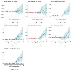
I also report estimates of the treatment effect on home values based on the number of bedrooms in a home, shown in Table 7. We can see that in high tourism zipcodes, the negative effect is driven by smaller homes with 3 bedrooms or less, and primarily by the 1-2 bedroom homes. These smaller homes have more revenue potential given that their smaller size appeals to tourists, which can explain the decrease in their value once restrictions on STRs are implemented. On the other hand, the positive treatment effect on low tourism zipcodes is mostly driven by large effects of around 3% on larger homes (3+ bedrooms). We can expect zipcodes with larger homes to experience more of a relative increase in noise, concern for safety, etc. associated with STRs as these areas typically appeal to families and those who prefer to have a stronger sense of community. There is also lower revenue potential for these homes, particularly in areas with low tourism levels as the location will be less attractive to tourists. Thus, for large homes in low tourism areas, we can expect that negative externalities of STRs are the dominant effect on home values, explaining the positive treatment effect we see. Also, note that all the mentioned and relevant estimates are significant at the 1% level, and we can see from the corresponding event study plots in Figures 7, 8, and 9 that there are no differential pretrends. Thus, the estimates in Tables 6 and 7 are valid and can be interpreted as casual effects.

6.3         Limitations

The main limitation in my analysis is that I cannot confirm whether STR regulations are affecting the housing market through a reduction in STR supply, as I am assuming throughout this paper, or another unexpected channel. However, previous literature has found that STR regulations were successful in reducing Airbnb supply so it is likely that this is true for my sample as well. I must still take into consideration, though, that the success of STR regulations found in previous literature may only apply to the specific cities in the analysis, and cannot be extrapolated to all 47 of the regulated cities in my sample.

Another limitation of my paper would be the minor pretrends we see in the majority of the event study plots. The best evidence in support of the parallel trends assumption would be no pretrend at all for any of my specifications. Despite the potential bias in my estimates of the treatment effect, it is clear from all the figures in this paper that the treatment effects are not primarily driven by these minor pretrends and grow much larger in magnitude as well. Therefore, if there was indeed any over- or under-estimation of the true effects, I believe they would not make a significant difference in my results. More importantly, the difference in the sign of the effect on low vs. high tourism areas would remain.

7           Conclusion

In this paper, I show that short-term rentals can have varying impacts on home values depending on characteristics of the neighborhood and of the home itself. STRs have the potential to increase home values if the location of the home is attractive to tourists and if the home is a suitable size for a short-term stay. However, in contrast to existing literature, I find that STR presence could actually decrease home values when the home is a single family home or is larger (3+ bedrooms), and in more local communities that do not cater towards tourists as much. I estimate that on average, STR regulations in the U.S. caused a 3.26% decrease in home values in high tourism zipcodes, with the effect being as high as 5.5% for 1 bedroom homes. In contrast, low tourism zipcodes experienced a 2.82% increase in home values as a result of the regulations, with slightly higher effects for larger homes in those neighborhoods. These findings have important implications for policymakers, many of whom have implemented STR regulations due to local affordability concerns. My results suggest, however, that these regulations may have the opposite effect than intended on local neighborhoods specifically, and will instead decrease home prices in areas already dominated by tourists.

In terms of more research on this topic, it would be insightful to explore the effects of STR regulation on rental prices further. Although I conducted additional analysis regarding the heterogeneous treatment effects of STR regulation on home values, I did not do the same for rental prices given the statistically insignificant overall treatment effect I found. It would be informative to find whether there truly is no effect of STR regulation on rentals when using a large sample of cities, or if there are any methods to better isolate this treatment effect. Additional analysis can also be done on whether the regulations considered in this paper actually affected the housing market through STR supply, as confirming the channel that is driving the causal effects I find in this paper will be important for making future policy decisions.

8           References

“About Us.” Airbnb Newsroom, n.d. https://news.airbnb.com/about-us/.

Athey, Susan, and Guido W. Imbens. “Design-Based Analysis in Difference-in-Differences Settings with Staggered Adoption.” Journal of Econometrics 226, no. 1 (2022): 62–79. https://doi.org/10.1016/j.jeconom.2020.10.012.

Barker, Gary. “The Airbnb Effect on Housing and Rent.” Forbes. Forbes Magazine, October 12, 2022. https://www.forbes.com/sites/garybarker/2020/02/21/the-airbnb-effecton-housing-and-rent/?sh=4cc53de02226.

Barron, Kyle, Edward Kung, and Davide Proserpio. “The Effect of Home-Sharing on House Prices and Rents: Evidence from Airbnb.” Marketing Science 40, no. 1 (2021): 23–47. https://doi.org/10.1287/mksc.2020.1227.

Bekkerman, Ron, Maxime C. Cohen, Edward Kung, John Maiden, and Davide Proserpio. “The Effect of Short-Term Rentals on Residential Investment.” Marketing Science, 2022. https://doi.org/10.1287/mksc.2022.1409.

Borusyak, Kirill, Xavier Jaravel, and Jann Spiess. “Revisiting Event Study Designs: Robust and Efficient Estimation.” SSRN Electronic Journal, 2022. https://doi.org/10.2139/ssrn.2826228.

Callaway, Brantly, and Pedro H.C. Sant’Anna. “Difference-in-Differences with Multiple Time Periods.” Journal of Econometrics 225, no. 2 (2021): 200–230. https://doi.org/10.1016/j.jeconom.2020.12.001.

Chen, Wei, Zaiyan Wei, and Karen Xie. “The Battle for Homes: How Does Home Sharing Disrupt Local Residential Markets?” Management Science 68, no. 12 (2022): 8589–8612. https://doi.org/10.1287/mnsc.2022.4299.

de Chaisemartin, Cl´ement, and Xavier D’Haultfœuille. “Two-Way Fixed Effects Estimators with Heterogeneous Treatment Effects.” American Economic Review 110, no. 9 (2020): 2964-96. https://10.1257/aer.20181169.

Duso, Tomaso, Claus Michelsen, Maximilian Scha¨fer, and Kevin Tran. “Airbnb and Rents: Evidence from Berlin.” SSRN Electronic Journal, 2020. https://doi.org/10.2139/ssrn.3676909.

Farhoodi, Abdollah, Nazanin Khazra, and Peter Christensen. “Does Airbnb Reduce Matching Frictions in the Housing Market?” SSRN Electronic Journal, 2021. https://doi.org/ 10.2139/ssrn.3923826.

Farronato, Chiara, and Andrey Fradkin. “The Welfare Effects of Peer Entry: The Case of Airbnb and the Accommodation Industry.” American Economic Review 112, no. 6 (2022): 1782–1817. https://doi.org/10.1257/aer.20180260.

Garcia-Lo´pez, Miquel-Angel, Jordi Jofre-Monseny, Rodrigo Mart´ınez-Mazza, and Mariona` Segu´. “Do Short-Term Rental Platforms Affect Housing Markets? Evidence from Airbnb in Barcelona.” Journal of Urban Economics 119 (2020): 103278. https://doi.org/10.1016/ j.jue.2020.103278.

Genesove, David, and Lu Han. “Search and Matching in the Housing Market.” Journal of Urban Economics 72, no. 1 (2012): 31–45. https://doi.org/10.1016/j.jue.2012.01.002.

Goodman-Bacon, Andrew. “Difference-in-Differences with Variation in Treatment Timing.” Journal of Econometrics 225, no. 2 (2021): 254–77. https://doi.org/10.1016/j.jeconom. 2021.03.014.

Guttentag, Daniel. “What Airbnb Really Does to a Neighbourhood.” BBC News. BBC, August 29, 2018. https://www.bbc.com/news/business-45083954.

Han, Lu, and William C. Strange. “The Microstructure of Housing Markets.” Handbook of Regional and Urban Economics, 2015, 813–86. https://doi.org/10.1016/b978-0-44459531-7.00013-2.

Horn, Keren, and Mark Merante. “Is Home Sharing Driving up Rents? Evidence from Airbnb in Boston.” Journal of Housing Economics 38 (2017): 14–24. https://doi.org/10.1016/j.jhe.2017.08.002.

“Housing Data.” Zillow, n.d. https://www.zillow.com/research/data/.

Koster, Hans R.A., Jos van Ommeren, and Nicolas Volkhausen. “Short-Term Rentals and the Housing Market: Quasi-Experimental Evidence from Airbnb in Los Angeles.” Journal of Urban Economics 124 (2021): 103356. https://doi.org/10.1016/j.jue.2021.103356.

Mortensen, Dale T. “Chapter 15 Job Search and Labor Market Analysis.” Handbook of Labor Economics, 1986, 849–919. https://doi.org/10.1016/s1573-4463(86)02005-9.

Sun, Liyang, and Sarah Abraham. “Estimating Dynamic Treatment Effects in Event Studies with Heterogeneous Treatment Effects.” Journal of Econometrics 225, no. 2 (2021): 175–99. https://doi.org/10.1016/j.jeconom.2020.09.006.

Valentin, Maxence. “Regulating Short-Term Rental Housing: Evidence from New Orleans.” Real Estate Economics 49, no. 1 (2020): 152–86. https://doi.org/10.1111/15406229.12330.

Zervas, Georgios, Davide Proserpio, and John W. Byers. “The Rise of the Sharing Economy:Estimating the Impact of Airbnb on the Hotel Industry.” Journal of Marketing Research 54, no. 5 (2017): 687–705. https://doi.org/10.1509/jmr.15.0204.

“ZIP Codes Business Patterns (ZBP) APIs.” United States Census Bureau, n.d. https:// www.census.gov/data/developers/data-sets/cbp-nonemp-zbp/zbp-api.2000.html#list-tab-2081829620.

Tables

Table 1: Summary Statistics – Short-Term Rental Regulations in U.S. Cities

	Mean	SD	Median	Min	Max	N
Regulated	0.43	0.50	0	0	1	110
Effective Date	214.66	20.45	220	151	240	47

Note: ‘Effective Date’ is displayed in terms of months since January 2000.

Table 2: Summary Statistics – Zillow Housing Data (Control Group)

	Mean	SD	Median	Min	Max	N
ZORI	1123.584	498.0112	1069.04	52.04023	3,610	43724
ZHVI	203257	148681.1	162516.5	31519	1,170,277	214566
Condo	174632.7	110950	145270	45157	953,906	111583
Single Family Home	216410.1	171206.5	167428.5	31040	1,448,761	212262
1 Bedroom	140956.9	91245.66	117423	29147	741,172	65602
2 Bedrooms	153045.1	107018.2	121849	27954	937,010	193326
3 Bedrooms	202406.1	152777.6	157626	32458	1,426,776	205848
4 Bedrooms	267781.3	207804.3	210253	35732	1,697,837	198043
5+ Bedrooms	398513.2	319765.7	312995	46727	2,541,424	152775

Notes: All values in this table are in USD. ZHVI – Zillow Home Value Index. ZORI Zillow Observed Rent Index.

Table 3: Summary Statistics – Zillow Housing Data (Treatment Group)

	Mean	SD	Median	Min	Max	N
ZORI	1445.51	712.6528	1298.692	52.04023	3,610	52976
ZHVI	298538.2	240129.4	220955	31519	1,170,277	246705
Condo	269294.4	193899.3	211868	45157	953,906	158246
Single Family Home	318251.5	283816.6	222935	31040	1,448,761	238895
1 Bedroom	233785.1	157279.6	195951	29147	741,172	112405
2 Bedrooms	247721.8	203612.7	175831	27954	937,010	223101
3 Bedrooms	316468	287638.3	210980	32458	1,426,776	235172
4 Bedrooms	374817.3	334212.7	260968	35732	1,697,837	221630
5+ Bedrooms	527282.9	485489.3	370058.5	46727	2,541,424	176166

Notes: All values in this table are in USD. ZHVI – Zillow Home Value Index. ZORI Zillow Observed Rent Index.

Table 4: Summary Statistics – Zipcode Tourism Levels in 2000

	Mean	SD	Median	90%	Min	Max	N
# Establishments	53.52	44.03	45	108	1	339	461024

Note: Tourism levels are proxied by the number of establishments in the accommodation and food services industries (NAICS Code 72).

Table 5: Treatment Effects of STR Regulation on Home Values (ln ZHVI) and Rents (ln ZORI) on All Homes

ln(ZHVI)                                                                                         ln(ZORI)

Overall ATT θ (All Zipcodes)	0.0198***	-0.0244
	(0.0042)	(0.0164)
Early Regulation Zipcodes	0.0226***	-0.0346
	(0.0049)	(0.0218)
Late Regulation Zipcodes	0.0209***	0.0137
	(0.0058)	(0.009)

Significance levels: ^*p < 0.1, ^**p < 0.05, ^***p < 0.01.

Note: ‘Early Regulation Zipcodes’ indicates that the treatment group only included zipcodes that were regulated before April 2018. Similarly, ‘Late Regulation Zipcodes’ only includes zipcodes that were regulated on or after April 2018 in the treatment group.

Table 6: Treatment Effects of Regulation on Home Values (ln ZHVI) by Home Type and

Tourism Level

All Homes                                                                       Condo

Overall ATT θ (All Zipcodes)	0.0198***	0.0104***	0.0266***
	(0.0042)	(0.006)	(0.0039)
High Tourism Zipcodes	-0.0326***	-0.0508***	-0.0122
	(0.0012)	(0.0136)	(0.0141)
Low Tourism Zipcodes	0.0282***	0.024***	0.0332***
	(0.0043)	(0.0072)	(0.0045)

Significance levels: ^*p < 0.1, ^**p < 0.05, ^***p < 0.01.

Notes: ‘High Tourism Zipcodes’ includes zipcodes belonging to the top decile of the sample in terms of establishments in the Accomodation and Food Services industries (NAICS Code 72), while the rest fall under the category ‘Low Tourism Zipcodes’.

Table 7: Treatment Effects of Regulation on Home Values (ln ZHVI) by Home Size and Tourism Level

	1 Bdrm	2 Bdrm	3 Bdrm	4 Bdrm	5+ Bdrm
Overall ATT θ (All Zipcodes)	-0.0019	0.0084	0.0230***	0.0256***	0.0294***
	(0.0078)	(0.006)	(0.0045)	(0.0041)	(0.0058)
High Tourism Zipcodes	-0.055***	-0.0514***	-0.0249*	-0.0123	0.0075
	(0.0175)	(0.0142)	(0.0135)	(0.0147)	(0.021)
Low Tourism Zipcodes	0.014*	0.0197***	0.0314***	0.0311***	0.0312***
	(0.0078)	(0.0062)	(0.0045)	(0.0046)	(0.0006)

Significance levels: ^*p < 0.1, ^**p < 0.05, ^***p < 0.01.

Note: ‘High Tourism Zipcodes’ includes zipcodes belonging to the top decile of the sample in terms of establishments in the Accomodation and Food Services industries (NAICS Code 72), while the rest fall under the category ‘Low Tourism Zipcodes’.

Figures

Figure 1: Distribution of Short-Term Rental Regulation Dates in U.S. Cities

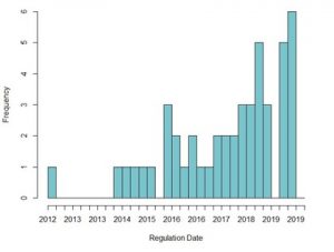
Figure 2: Distribution of Zipcode Tourism Levels^* in 2000

^*Tourism levels are proxied by the number of establishments in the accommodation and food services industries.

Figure 3: Treatment Effects on Home Values (ZHVI) & Rental Prices (ZORI) Over Time

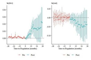
Figure 4: Treatment Effects on Home Values (ZHVI) by Regulation Time

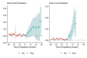
Figure 5: Treatment Effects on Rental Prices (ZORI) by Regulation Time

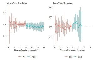
Figure 6: Treatment Effects on Home Values (ZHVI) by Tourism Level

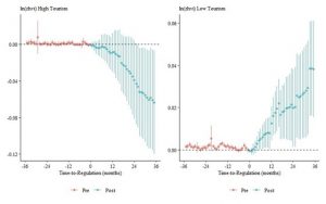
Figure 7: Treatment Effects on Home Values (ZHVI) by Home Type/Size

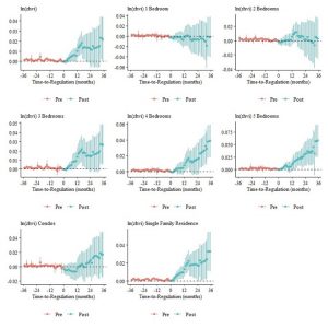
Figure 8: Treatment Effects on ZHVI by Home Type/Size – High Tourism

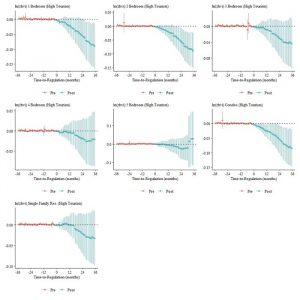
Figure 9: Treatment Effects on ZHVI by Home Type/Size – Low Tourism

Appendix A

Table A1: Summary Statistics – Zillow Housing Data for High Tourism Zipcodes (Control Group)

	Mean	SD	Median	Min	Max	N
ZORI	1348.049	522.995	1246.971	52.04023	3,610	5075
ZHVI	267376.2	177132.1	216262	31519	1,170,277	24035
Condo	201576.9	139793	160223	45157	953,906	16859
Single Family Home	301286.7	220149.9	234366	31040	1,448,761	23215
1 Bedroom	167240	98230.87	137629	29147	492,498	10489
2 Bedrooms	216893.7	142698.7	171033	34472	831,309	20098
3 Bedrooms	290144.5	216626.5	210659.5	32458	1,426,776	22278
4 Bedrooms	372707.9	287399.4	275334.5	35732	1,697,837	20630
5+ Bedrooms	545108.6	470133.9	375313.5	59905	2,541,424	17416

Notes: All values in this table are in USD. ZHVI – Zillow Home Value Index. ZORI Zillow Observed Rent Index.

Table A2: Summary Statistics – Zillow Housing Data for High Tourism Zipcodes (Treatment Group)

	Mean	SD	Median	Min	Max	N
ZORI	1808.209	786.2503	1645.24	52.04023	3,610	8109
ZHVI	422269.1	290091.2	334109	53481	1,170,277	35907
Condo	358588.7	236967.6	301456.5	45157	953,906	29906
Single Family Home	472677	371510	348448	51687	1,448,761	33769
1 Bedroom	304293.5	183412.8	255686.5	37024	741,172	24448
2 Bedrooms	387770.8	259523.3	316423	27954	937,010	32145
3 Bedrooms	511492.5	397760.5	362956	37637	1,426,776	32967
4 Bedrooms	586507.4	468895.7	407554	59604	1,697,837	28032
5+ Bedrooms	792787.4	691911.9	512523.5	68888	2,541,424	22474

Notes: All values in this table are in USD. ZHVI – Zillow Home Value Index. ZORI Zillow Observed Rent Index.

Table A3: Summary Statistics – Zillow Housing Data for Low Tourism Zipcodes (Control Group)

	Mean	SD	Median	Min	Max	N
ZORI	1094.11	487.0192	1048.035	52.04023	3,610	38649
ZHVI	195168.6	142663.3	155930	31519	1,170,277	190531
Condo	169837.1	104262.7	143078	45157	953,906	94724
Single Family Home	205987.2	161141.1	159543	31040	1,448,761	189047
1 Bedroom	135954.8	88980.64	112812	29147	741,172	55113
2 Bedrooms	145637.4	99455.59	117982.5	27954	937,010	173228
3 Bedrooms	191758.2	139396	151266	32458	1,426,776	183570
4 Bedrooms	255580.1	192796.8	202443	35732	1,697,837	177413
5+ Bedrooms	379651.5	289566	305114	46727	2,541,424	135359

Notes: All values in this table are in USD. ZHVI – Zillow Home Value Index. ZORI Zillow Observed Rent Index.

Table A4: Summary Statistics – Zillow Housing Data for Low Tourism Zipcodes (Treatment Group)

	Mean	SD	Median	Min	Max	N
ZORI	1379.958	678.1417	1244.427	52.04023	3,610	44867
ZHVI	277462.1	223826.1	204446	31519	1,170,277	210798
Condo	248486.9	176017.8	194604.5	45157	953,906	128340
Single Family Home	292829.1	257914	206883.5	31040	1,448,761	205126
1 Bedroom	214187	143166.2	179604	29147	741,172	87957
2 Bedrooms	224146.4	182323.7	161894	27954	937,010	190956
3 Bedrooms	284671.6	251433.3	195298	32458	1,426,776	202205
4 Bedrooms	344165.7	297673	246972.5	35732	1,697,837	193598
5+ Bedrooms	488458.8	433990.7	356273.5	46727	2,541,424	153692

Notes: All values in this table are in USD. ZHVI – Zillow Home Value Index. ZORI Zillow Observed Rent Index.

Return to the Department of Economics website. 

Scroll more news.